Statistics

Poisson Statistics

The most important error is the statistical fluctuation that stems from the randomness of the scattering events. Counts of such events follow the Poison distribution. Such, the error (\(\sigma\)) is \(\sqrt n\) for a count of \(n\). The result of which is, that the relative error \(\frac{\sqrt n}{n}\) rapidly gets small for larger counts.

Each Pixel in the SAXS sensor counts the number of events, and thus follows the Poisson statistics. The error of a sum of pixels is calculated as.

\[\sigma_{sum}=\sqrt{\sum_i \sigma_i^2}\]

which means here

\[\sigma_{sum}=\sqrt{\sum_i n_i}\]

Rescaled over the number of pixels (\(P\)) in the sum this gives:

\[\sigma_{sum}=\frac{\sqrt{\sum_{i=1}^P n_i}}{P}\]

The SAXS.calibration.plot() method of the SAXS.calibration class will give you the Poisson error along with the standard deviation. So for regions, where the total number of counts is too small, you can see if there is a significant error. This might occur, if too few pixels are used for a data point or the intensity is just to small.

Standard Deviation

The standard deviation of the mean that is taken through the integration is not as such particularly useful to estimate the error of the resulting intensities because there are quite a few things that produce an angle dependence. In an optimal case, if the angle dependence can be corrected with the Polarization correction, the standard deviation of the integration might be very small. In an ordinary case the standard deviation gives you a measure of how spread the intensities within a radius interval are.

(Source code, png, hires.png, pdf)

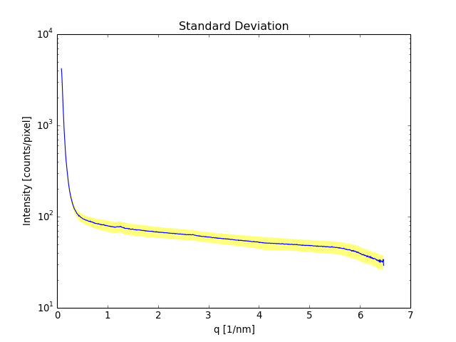
The standard deviation is bright yellow and the Poison error is blueisch

(Source code, png, hires.png, pdf)

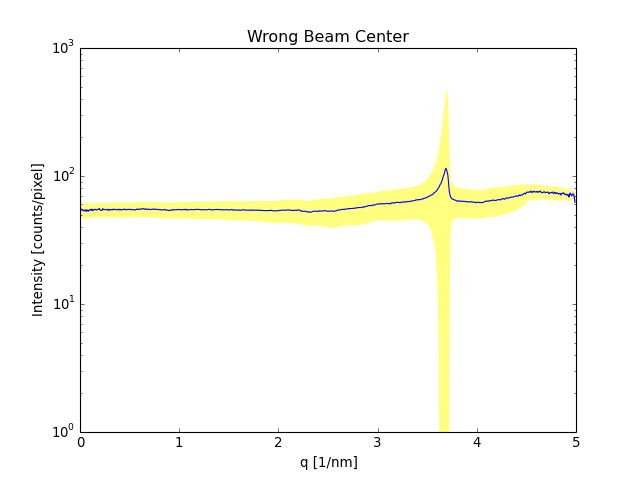
If the calibration is wrong you will for example see in the standard deviation. Like in this example. Here the beam center is wrong.