The Geometry
The plane of the sensor is not perfectly normal to the beam. So in order to calculate witch pixel is on witch cone in the diffracted light, we need to express the geometry somehow.
Every pixel has the polar coordinates \(r\), \(\phi\) with the projected diffraction center in the origin. For each pixel (P) the triangle S,C,P (Sample, Center, Pixel, \(\theta\), \(\beta\), \(\gamma\)) can be fully expressed with the law of cosines.

The SCP triangle.
\(l\) is the distance the light travels from the diffraction center to the sensor.
\(r\) is the radial coordinate of the pixel P.
from these two formulas the diffraction angle (here) \(\theta\) can be computed.

Angle between two planes.
\(\alpha\) comes from the following relation in figure Angle between two planes.
The angle between the sensor plane and the normal plane to the ray is given by \(\tau\). The slope \(s\) derived from \(\tau\) is
On the (red) unit circle in the plane of the sensor the distance to the plane normal to the ray is expressed as
The angle \(\alpha\) is therefore:
in Python code this is SAXS.calc_theta():
def calc_theta(r,theta,d,tilt,tiltdir):
   alpha=np.arcsin(np.sin(tilt)*np.sin(theta+tiltdir))
   lsquared=d**2 +r**2 -2*d*r*np.cos(np.pi/2+alpha)
   return np.arccos(-(r**2-lsquared-d**2)/(2*np.sqrt(lsquared)*d))
This angle \(\theta\) then is calculated for every sub pixel in the sensor. This number then can be rescaled and rounded to the nearest integer in order to get unique integer labels for all the pixels. This labels are the index of the radial interval.
Tilt Angle Correction Test
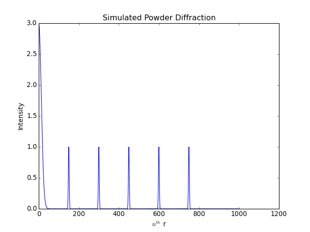
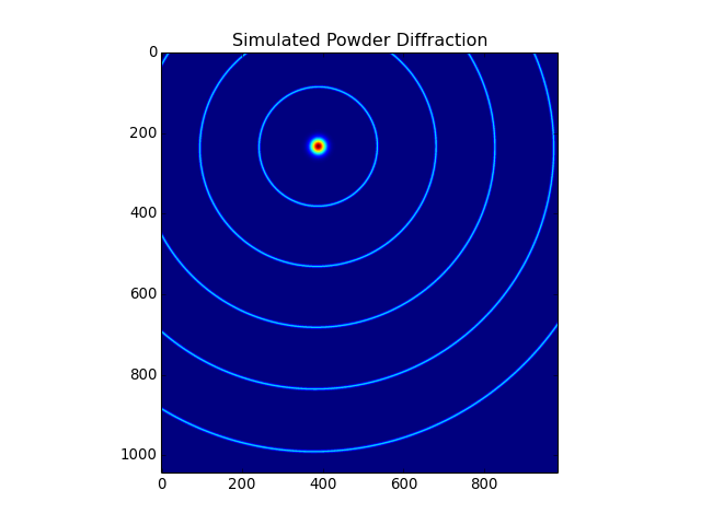
To check if the tilt angle correction is working, lets create some fake calibration data, with the following peaks in the diffraction curve:
(Source code, png, hires.png, pdf)
(Source code, png, hires.png, pdf)
This was done with this configuration file:
{
    "Geometry": {
        "Tilt": {
            "TiltAngleDeg": -10,
            "TiltRotDeg": 73.569
        },
        "DedectorDistanceMM": 1031.657,
        "BeamCenter": [
            808.37,
            387.772
        ],
        "Imagesize": [
            1043,
            981
        ],
        "PixelSizeMicroM": [
            172.0,
            172.0
        ]
    },
    "Directory": [
        "."
    ],
    "Masks": [
        {
            "PixelPerRadialElement": 1,
            "MaskFile": "emptymask.tif",
            "Oversampling": 2,
            "qStart": 0.0,
            "qStop": 5.0
        }
    ],
    "Wavelength": 1.54
}
Which amounts to a large tilt, lets see what Fit2d makes of it
INFO: SOLUTION 2
INFO: Best fit beam centre (X/Y mm) =   66.78356      138.9544
INFO: Best fit beam centre (X/Y pixels) =   388.2765      807.8745
INFO: Cone  1 best fit 2 theta angle (degrees) =   1.392646
INFO: Cone  2 best fit 2 theta angle (degrees) =   2.780810
INFO: Cone  3 best fit 2 theta angle (degrees) =   4.168858
INFO: Cone  4 best fit 2 theta angle (degrees) =   5.556975
INFO: Cone  5 best fit 2 theta angle (degrees) =   6.944765
INFO: Best fit angle of tilt plane rotation (degrees) =   73.59509
INFO: Best fit angle of tilt (degrees) =  -10.00601
INFO: Estimated coordinate radial position error (mm) =  0.7136476E-02
INFO: Estimated coordinate radial position error (X pixels) =  0.4149114E-01
Seems OK.